On the Las Vegas Strip, the average return rate for slot machines is approximately 93%, meaning that for every $1 wagered, players typically receive only $0.93 back; on Polymarket, traders voluntarily accept returns as low as $0.43 for a $1 bet on underdog outcomes with odds even worse than those in casinos.

This is not metaphorical—it’s grounded in real data. Researcher Jonathan Becker conducted an analysis of all settled markets on Kalshi, covering 721 million transactions and $18.26 billion in trading volume. The patterns he identified apply equally to Polymarket—identical mechanisms, identical biases, and thus identical opportunities. The data reveals a clear conclusion: approximately 87% of prediction market wallets ultimately lose money, but the remaining 13% do not win by luck—they master a mathematical framework most traders have never even heard of.

This article dissects five game-theoretic formulas that separate winners from losers, each accompanied by its underlying mathematics, real-world case studies, and executable Python code. Traders already applying these methods include:

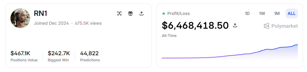
• RN (Polymarket address: https://polymarket.com/profile/%40rn1): A Polymarket algorithmic trading bot that has generated over $6 million in cumulative profit using the models described, primarily in sports markets.

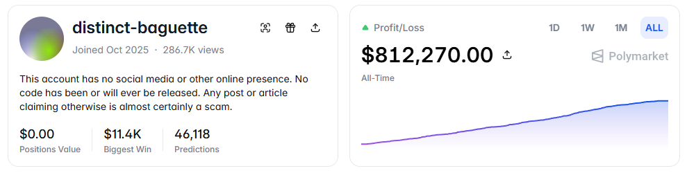
• distinct-baguette (Polymarket address: https://polymarket.com/profile/%40distinct-baguette): Turned $560 into $812,000 by providing liquidity in UP/DOWN markets.

I. Expected Value: The Core Formula

Every transaction on Polymarket is fundamentally a judgment of expected value. Most traders rely on intuition, while the top 13% make decisions based on math. Expected value (EV) measures not the outcome of a single event, but the average return over repeated trials, serving as a criterion for determining whether a trade is worth entering.

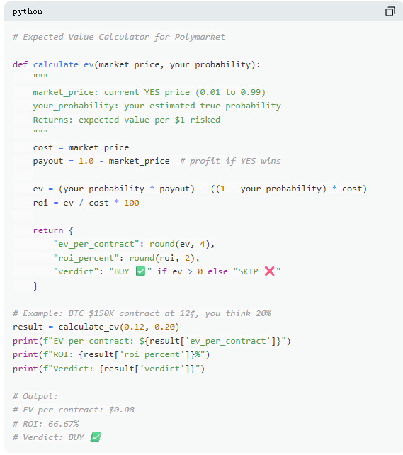
Take a real market example: “Will Bitcoin reach $150,000 before June 2026?” The current YES price is 12¢, implying a 12% market-embedded probability. Based on on-chain data, halving cycles, and ETF inflows, suppose the true probability is estimated at 20%. This trade then has positive EV. Calculating this, each contract purchased at 12¢ yields an average gain of 8¢ over time. Buying 100 contracts at a cost of $12 results in an expected return of $8—a return rate of approximately +66.7%.

Yet data shows most prediction market traders don’t perform such calculations. Among a sample of 72 million trades, takers (market buyers) lost about 1.12% per trade on average, while makers (limit order providers) gained about 1.12% per trade. The gap isn’t due to information asymmetry but patience—makers wait for positive EV opportunities, whereas takers are more prone to impulsive trading.

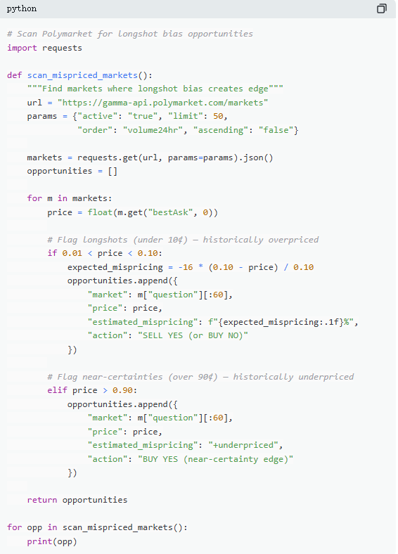
II. Mispricing: The Low-Price Trap

“Underdog bias” is one of the most costly errors in prediction markets—traders systematically overvalue low-probability events, paying excessive prices for contracts that appear cheap. A 5¢ contract should theoretically have a 5% win rate, but on Kalshi, the actual win rate is only 4.18%, resulting in a -16.36% pricing deviation. In more extreme cases, a 1¢ contract should imply a 1% chance, yet for takers, the actual win rate is just 0.43%, with a deviation of -57%.

Overall, the market pricing is relatively accurate in the mid-range (30¢–70¢), but significant deviations emerge at both ends: contracts priced below 20¢ consistently exhibit lower actual win rates than implied probabilities, while those above 80¢ tend to have higher win rates than their quoted prices suggest.

In other words, inefficiency is concentrated at the extremes—precisely where emotional trading dominates. Two key formulas capture this:

Formula One: Mispricing (δ)

Mispricing quantifies the divergence between a contract’s actual win rate and its implied probability. Take a 5¢ contract: among 100,000 completed trades at that price, if 4,180 resulted in YES, the actual win rate is 4.18%, compared to the 5.00% implied by the price. The difference is -0.82 percentage points, or a relative deviation of approximately -16.36%. This means every purchase of a 5¢ contract effectively pays a premium of about 16.36%.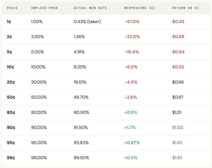

Formula Two: Gross Excess Return (rᵢ)

While mispricing reflects aggregate bias, gross excess return reveals the actual return structure of individual trades—where behavioral biases become evident. When buying a 5¢ contract, two outcomes arise: if it wins, the return reaches +1,900% (roughly 20x); if it loses, the entire 5¢ stake is forfeited.

This explains why underdog bets are so attractive—the high upside is memorable, amplified, and widely shared. But overall, the actual win rate falls short of the price-implied probability, and the asymmetric structure between total loss and massive gain leads to negative expected value across many trades—effectively equivalent to buying overvalued lottery tickets.

The bias exhibits a clear price gradient: the cheaper the contract, the worse the actual return. For instance, as a taker, every $1 invested in a 1¢ contract averages only $0.43 back, whereas $1 in a 90¢ contract yields about $1.02 on average. Lower prices correspond to worse execution conditions.

Further role segmentation reveals this structure is nearly mirror-like: taker losses in low-price zones (as low as -57%) directly correspond to maker gains in the same range; overall market mispricing lies between them. In essence, every dollar lost by a taker is captured by a maker.

From a game-theoretic perspective, low-probability contracts are systematically overpriced, while high-probability ones are often underpriced. The true strategy is not chasing underdogs—but selling them and buying high-conviction outcomes.

III. Kelly Criterion: How Much to Bet

Once a positive EV opportunity is identified, the real challenge begins: how much to bet? Overbetting can wipe out weeks of profits with a single loss; underbetting, even with an edge, leads to negligible growth. Between “going all-in” and “not betting at all,” there exists a mathematically optimal bet size—the Kelly Criterion.

Proposed by John L. Kelly Jr. in 1956 originally for optimizing signal-to-noise ratios in communications, the Kelly Criterion was later proven to be one of the most effective position-sizing strategies in gambling, trading, and prediction markets. Professional poker players, sports bookies, and Wall Street quant funds almost universally employ some form of Kelly-based strategy.

In prediction markets, due to binary contracts (paying $1 or $0) and prices reflecting probabilities, the Kelly formula applies directly. The key is understanding the odds (b): buying a YES contract at 30¢ means risking $0.30 for a potential $0.70 gain, yielding odds of 0.70 / 0.30 ≈ 2.33; at 50¢, odds are 1; at 10¢, they’re 9; at 80¢, only 0.25. The higher the odds, the larger the suggested bet size under Kelly, provided there is an edge.

A critical principle: never use full Kelly. While full Kelly maximizes long-term capital growth mathematically, it entails extreme volatility—drawdowns often exceed 50%. Although it may yield the highest final equity curve over long periods, the severe fluctuations frequently deter most traders from holding through. Thus, practitioners commonly use fractional Kelly (e.g., 1/2 or 1/4 Kelly). For example, full Kelly produces the steepest growth curve but the highest volatility; 1/4 Kelly offers smoother growth with controlled drawdowns; 1/2 Kelly sits between the two.

Ultimately, the Kelly Criterion provides a disciplined framework: first determine whether an edge exists (i.e., subjective probability exceeds market-implied probability), then decide capital allocation. Only when both “whether to bet” and “how much to bet” are mathematically constrained does trading transition from gambling to strategy.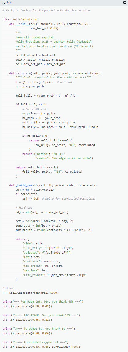

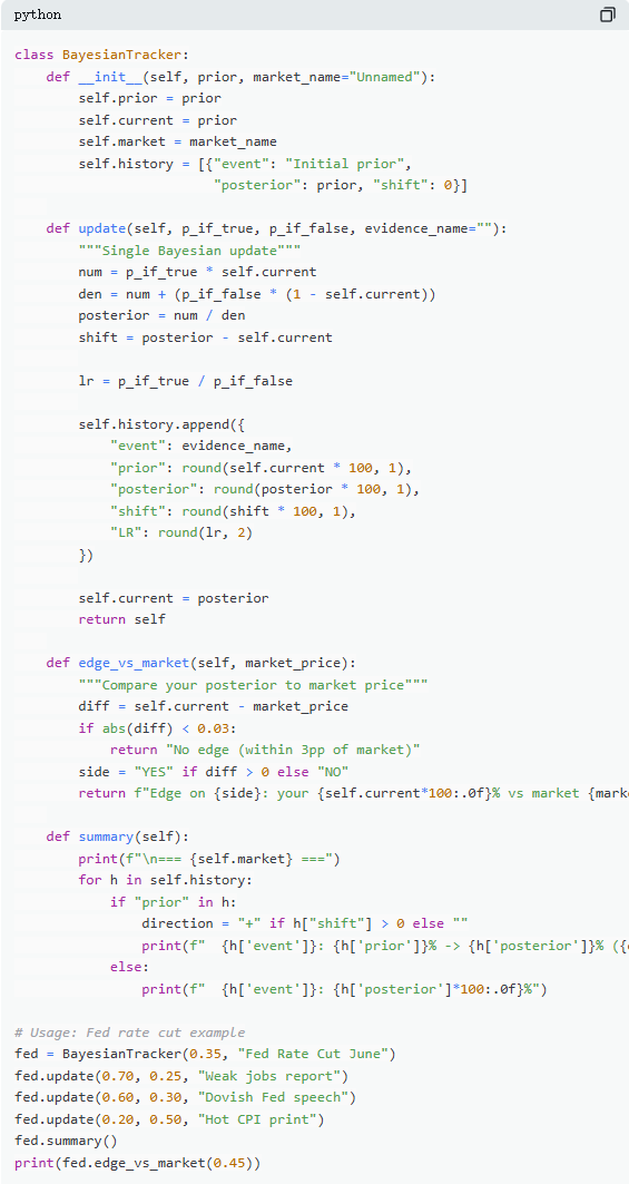
IV. Bayesian Updating: Think Like an Expert

The reason prediction markets fluctuate is because new information constantly enters. The key isn’t whether your initial assessment was correct, but how you adjust your beliefs when evidence changes. Most traders either ignore new information or overreact—Bayesian updating provides a mathematical method for determining “how much adjustment is appropriate.”

At its core, the logic simplifies to: New belief = (Evidence support for hypothesis × Prior belief) ÷ Overall likelihood of evidence occurring. In practice, this is often expanded via the law of total probability into a computationally tractable form.

Consider a typical market: “Will the Fed cut rates at the June meeting?” The current market price is 35¢, implying a 35% probability—an initial belief. Then, nonfarm payroll data releases: only 120,000 jobs added (expected 200,000), unemployment rises, wage growth slows. In this scenario, if the Fed actually cuts, the likelihood of weak employment data is high—estimated at 70%; if no cut occurs, such data still has a non-negligible chance—estimated at 25%.

Plugging into Bayesian updating, the revised probability becomes approximately 60.1%—a jump from 35% to 60.1%, an increase of about 25 percentage points. This demonstrates how a single piece of key information can significantly shift market expectations.

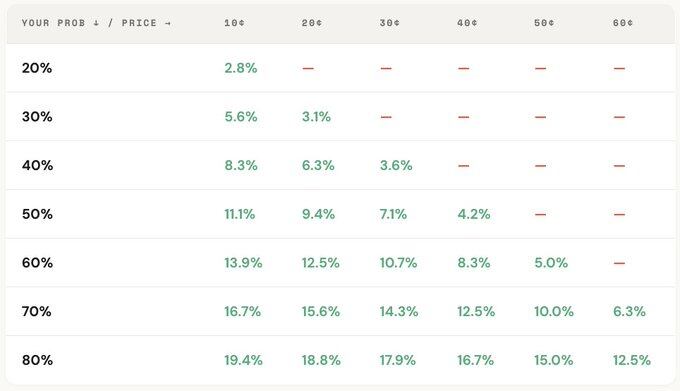
In practice, complete formula computation isn’t always needed. A more common approach is using the “likelihood ratio.” The same piece of evidence (e.g., LR = 3) impacts different starting beliefs differently: from 10%, it might raise to ~25%; from 50%, to 75%; from 90%, only to ~96%. The higher the initial uncertainty, the greater the impact of new information.

Long-term outperformers in prediction markets aren’t necessarily the most accurate predictors—but those who adapt fastest and most rationally to new evidence. Bayesian methods essentially provide a metric for “adjustment speed.”

V. Nash Equilibrium: The “Poker Formula” in Prediction Markets

In poker, bluffing is never arbitrary—it’s a precise, calculable strategy. There exists an optimal bluff frequency; deviating from it allows skilled opponents to exploit the imbalance. The same logic applies to prediction markets. On Polymarket, “bluffing” corresponds to contrarian trading—positioning against market consensus when pricing is biased; “folding” resembles passive taker behavior, continuously paying premiums for market sentiment.

On Polymarket, makers and takers form a similar adversarial relationship. Contrarian trading (opposing consensus) mirrors bluffing; trend-following (aligning with mainstream views) resembles value betting. From an equilibrium perspective, the market should render marginal participants indifferent between being a maker or a taker—this state defines the Nash equilibrium in prediction markets.

But this equilibrium is not static—it dynamically adjusts with participant composition. Data shows different market categories favor distinct optimal strategies: in more rational, efficiently priced domains (e.g., financial markets), contrarian space is limited; in emotionally charged, irrational-heavy areas (e.g., entertainment, sports), pricing inefficiencies are more prevalent, creating opportunities for contrarian strategies.

Even more crucially, this equilibrium evolves over time. Early (2021–2023), takers were profitable—optimal strategy favored active trading. After a surge in trading volume in Q4 2024, professional market makers entered en masse, altering market structure. The equilibrium shifted toward maker dominance (~65%–70%). This is a classic game-theoretic outcome: when participant structure changes, optimal strategy evolves. Strategies once effective in a “novice environment” rapidly fail against professional counterparts, forcing constant iteration of market “playbooks.”

Summary

87% of prediction market wallets ultimately lose money—not because the market is manipulated, but because traders never truly calculate. They buy underdog contracts at worse prices than slot machines, decide position sizes by gut feeling, ignore new information, and pay for “optimism” in every market-order transaction.

The 13% who sustain profitability aren’t luckier—they treat these five formulas as an integrated system, forming a complete workflow from judgment to execution, with every step anchored in 721 million real trades.

This window won’t last forever. As professional market makers enter, spreads are rapidly compressing: in 2022, takers had a ~+2.0% edge; today, that has flipped to -1.12%.

The question is simple: will you evolve with the market—or keep betting $1 for a $0.43 return on a lottery ticket?